
By Andrea Corvi
Canon vs Nikon and iOS vs Android are just two modern examples of “dualisms” that divide crowds.
The long-lasting Frequentist vs Bayesian fight is not any different and like the other two examples above, it’s still far from finding a winner.
This doesn’t affect just the CRO world but the same type of debates animate even the clinical trials and AI industry.
With this post, expect to:
- Understand the main differences between Frequentist and Bayesian
- See the two methodologies applied in R to analyse a real test
- Get an alternative answer to the million-dollar question: “Which one is better”?
This article, in fact, is not looking to find an ultimate winner nor discuss the statistics behind the two approaches (I’m an experimenter, not a statistician) but just share a few thoughts (coming from the practical application) on how you might leverage both approaches in your favour.
Let’s start by quickly reviewing and highlighting the main differences between the two schools of thought.
Context
When analysing experiments and sharing the test results with the business, we are trying (as experimenters) to understand what would happen if we were to push live the variation instead of control.
From a statistical point of view, we are using data analysis to infer the properties of the entire population (our users) from sample data (users that took part in the test): this is called statistical inference.
There are two general philosophies for inferential statistics, i.e. Frequentist and Bayesian.
How do these two translate in practical application?
Frequentist
The usual process consists of four steps:
- Formulate the null hypothesis Ho (“there is no difference between control and variation’s conversion rates”) and the alternative hypothesis Ha (“there is a difference between control and variation’s conversion rates”).
- Determine, prior to launching the test, the sample size needed to reach statistical significance given a minimum detectable effect and a power level.
- Launch the experiment and start collecting the data.
- Stop the test when the sample needed has been reached, compute the p-value (p) and compare the p to an acceptable significance level ? (typically 0.1 or lower to get 90% confidence level or higher). If p < ?, it means that the observed effect is statistically significant at the confidence level chosen, the null hypothesis is ruled out, and the alternative hypothesis is valid.
Inputs:
- Confidence Level
- Statistical Power
- Baseline Conversion Rate
- Minimum Detectable effect
Output:
- P-Value
- Confidence Intervals
Question Answered:
- Can we conclude that there is a difference between control and variation?
Bayesian
The usual process consists of three steps:
- Determine the prior distribution for the primary metric (typically conversion rate)
- Set the loss threshold: the maximum expected loss willing to accept if we were to make a mistake in concluding the experiment. The loss threshold makes us confident that the conversion rate wouldn’t drop more than an amount we’re comfortable with if we were wrong.
- Finally, collect the samples through a randomised experiment and use them to update the distribution about the conversion rate for control and variation. These are called the posterior distributions and will be used to calculate the probability that variation is better than control and the expected loss of making the wrong call.
Inputs:
- Prior distribution
- Loss threshold
- Data collected during the test
Outputs:
- The Probability that variation is better than control for the chosen metric
- Confidence intervals
- The Expected loss for each variation
Questions Answered:
- What’s the probability that variation is better than control?
- What would be the expected loss if we deploy variation instead of control?
Members of Experiment Nation’s Directory get promoted throughout our site and get access to our Online Bayesian A/B Test Calculator. Join our Directory today.
Main criticisms to both schools of thought
| ? Frequentist | ? Bayesian |
| • Treats the population parameter (conversion rate) for each variant as an unknown constant, whereas the Bayesian approach models each parameter as a random variable with some probability distribution instead • Slower to reach conclusions: it requires a fixed sample size and it’s dependent on the chosen minimum detectable effect. • Suffers from peeking problem (using statistical significance as a stopping rule instead of sample size)- not allowed by the purist frequentist methodology • Terminology (p-value, statistical significance, …) can be difficult to understand for the business | • Choosing the prior is subjective, and it affects test duration • Not immune to peeking • Data to choose the prior distribution is not always available • The concept of loss is not easy to communicate to the business |
In practice: Frequentist vs & Bayesian
Experimentation is a methodology that helps to mitigate the risk of making changes to a product, that’s why I’ve always approached both frequentist and bayesian as “tools” to reach the end goal: making as many correct decisions (for the users and the business) as possible.
In my experience, the choice on when to use either Frequentist or Bayesian comes down to mainly three factors:
- Test duration (time)
Frequentist relies on a minimum sample size that you need to collect before pausing the test (you are not allowed to skip this step). Yes, you can make good use of group sequential testing but there’s a trade-off to pay in terms of samples needed at every checkpoint. If the test is a good one you might be able to early-stop but in the case of smaller than expected lifts, it might just delay the stopping time.
Bayesian instead, does not require you to calculate the sample size prior to launching the experiment (as the stopping rule here is the loss threshold). You can still calculate it though (good practice) to avoid running the test for an unexpectedly long time.
Once you have these two potential test duration times, you might want to choose the one that will reach conclusions faster.
In my personal experience, Bayesian has been quite handy when running experiments on lower traffic volume pages as it often brought the test duration down to an acceptable amount.
- Support you can get from data scientists/analysts
I find the Bayesian methodology to be more “complex” to apply without the help of data scientists/analysts. Choosing the right prior, setting the right loss threshold requires a stronger statistical background compared to the frequentist approach.
Having dedicated people in your team (especially if proficient in R/Python and data manipulation) that can help experimenters to design and analyse experiments might be the crucial factor in adopting one (Bayesian) or the other (Frequentist) approach.
- How much you know about your primary metric
In the Bayesian school of thought, probabilities are fundamentally related to their knowledge about an event. Applying the Bayesian framework for a test where there’s no historical data about the main KPI might lead to inaccurate conclusions. Hence, in this case, frequentist might be a safer option.
Practical application
Let’s see how to analyse an experiment with both methodologies in R (script attached) using a real experiment’s data.
The baseline conversion rate that I started from was 41%, the goal was to increase it by at least 2%.
Frequentist
What do we know about the experiment? These were my pre-test choices:
- Minimum detectable effect I wanted to detect: 2%
- Power level: 80%
- Confidence Level: 95%
How many samples are necessary before concluding the test?
Just a little more than 15k sessions (calculated using power.prop.test in R).
Fast forward to a couple of weeks later and I had the necessary amount of data required (23744 sessions) so I paused the test.
This is how users reacted to both experiences:
control_visitors <- 11855
variation_visitors <- 11889
control_conversions <- 4926
variation_conversions <- 5080
The relative difference in conversion rates (in favour of variation): ~2.8%
Let’s use R again (this time prop.test) to find out the p-value.
P-value is 0.0332, smaller than our significance level of 0.05 so the difference measured during the test is statistically significant.

Bayesian
Same test as before, just a different methodology applied.
In this case, I had to first define a prior distribution – what do I knew about the metric I was trying to improve?
- It’s boolean (converted/non converted – 1,0)
- Its baseline conversion rate: 41%
As recommended by experts in the statistic field, I could then treat each conversion rate as a Bernoulli random variable and use the conjugate prior of the Bernoulli distribution Beta distribution as conjugate prior.
“I typically take a prior distribution that’s slightly weaker than the historical data suggest.” -Blake Arnold
Tweet
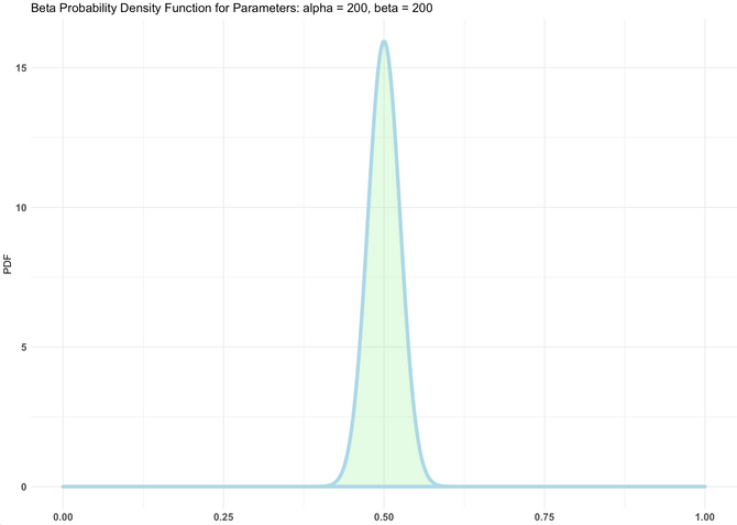
After plotting a few beta functions, it seemed that Beta(120,200) might have worked well to model the metric of the test.

I then used the R package BayesAB to make the magic happen. Once inputted the data and parameters required, this was the output:
- Probability that variation is better than control: 96.5%
- Interval: [0.25%,5.33%]
- Expected Loss probability for choosing variation over control: 0.0207%
The R script used to write this post can be found at the bottom of the page. It’s quite light and not commented but it covers all the frequentist and bayesian calculations I’ve made.
I’ll also link to another article I’ve written to share a more comprehensive frequentist R script ? here
What were the two analyses suggesting?
Both methodologies agreed: it’s worth (and low risk) adopting Variation instead of Control.
Would any of the two methodologies have performed better in terms of test duration?
In the pure frequentist approach, peeking is not allowed. This means that the duration is decided beforehand, through the estimation of the number of samples required to:
- detect the desired (or bigger) effect
- achieve the required level of significance and power
The test duration in the case of the pure frequentist application would have been a little more than 15k sessions (as calculated above).
In order to perform a better side by side comparison, I decided to use Group Sequential Testing: a frequentist approach that allows peeking at specific pre-determined checkpoints.
This allowance comes at the price of using stricter significance thresholds at each of the checkpoints and if it fails to early stop an experiment, it typically requires a higher amount of samples than pure frequentist.
For the comparison I’ve decided to use 3 different checkpoints (listed below) where I could check if either GST Frequentist or Bayesian would have allowed me to stop the test.
Peeking checkpoints:
- 6510 samples
- 16272 samples
- 23744 samples (test paused)
Frequentist GST
In none of these 3 points in time, under the GST stopping rules we would have been allowed to early stop the test (we didn’t cross either the red or green area).

Bayesian
In this case, how much the business is willing to risk on the metric plays a crucial role in the test duration. The reason is that being the expected loss threshold a crucial value in deciding when to stop the test, choosing a more or less conservative one directly impacts the duration.
Checkpoint 1 – at 6510 samples:
- Probability that variation is better than control: 73.5%
- Expected Loss: 0.456%
Checkpoint 2 – at 16272 samples:
- Probability that variation is better than control: 80.5%
- Expected Loss: 0.197%
Checkpoint 3 – at 23744 samples:
- Probability that variation is better than control: 96.5%
- Expected Loss: 0.0207%
Let’s now compare these values against the stopping threshold.
Stopping Threshold: The maximum expected loss willing to accept if you were to make a mistake in drawing conclusions from the experiment.
A More Conservative Threshold (willing to risk a 3% relative loss) ? 0.012%
A Less Conservative Threshold (willing to risk a 8% relative loss) ? 0.032%
The less conservative business would have stopped the test at checkpoint 3.
The more conservative business wouldn’t have stopped the test and kept it running.
Disclaimer: Test duration is highly influenced by some parameters that we have the freedom to choose. The Loss function used in GST or the loss threshold we set for Bayesian has a direct impact on when we can or cannot stop the test. A very interesting article (for Bayesian) on this topic by Blake Arnold can be found here.
Answer: In this example neither Bayesian nor Frequentist GST would have stopped the test earlier than I did with pure frequentist. If the effect would have been of higher magnitude than expected (e.g. 8% lift), then results might have been more interesting to compare.
Conclusions
In the CRO world, Bayesian and Frequentist are two alternative routes to the same destination: making a decision on a change.
Sometimes they cross, sometimes they overlap, sometimes they divert.
So here comes the one-million dollar question: which one should I use?
Short answer: BOTH, depending on the circumstances.
I’m personally more familiar with the Frequentist approach as it’s the one I started analysing tests with, and I’ve refined the application over the years (e.g. its group sequential testing variant).
Bayesian on the other hand is a very powerful alternative that is recommended in scenarios where you either have strong statistical skills or a team of data scientists/analysts that can guide the design and analysis of the experiments.
In my practical experience, Bayesian helped to run experiments in conditions where Frequentist wouldn’t have made it possible (due to a big gap between traffic levels and sample size required). On top of that, given that Bayesian always provides the probability of variation being better than control, making a decision (either to go live with the change or not) in cases where the test is not a clear winner, might be easier for the experimenter and the stakeholders involved.
Producing accurate and robust test analyses is a very hard task for every team: this is why mastering every possible available option becomes a success factor for any company that wants to run high velocity & high quality experimentation programs.
References and Interesting reads
https://towardsdatascience.com/bayesian-ab-testing-part-i-conversions-ac2635f878ec
https://towardsdatascience.com/bayesian-ab-testing-part-iii-test-duration-f2305215009c
https://towardsdatascience.com/exploring-bayesian-a-b-testing-with-simulations-7500b4fc55bc
https://blog.analytics-toolkit.com/2020/frequentist-vs-bayesian-inference/
http://ethen8181.github.io/Business-Analytics/ab_tests/frequentist_ab_test.html#power-analysis
R Script – with simulated data for side by side comparison
Frequentist – Bayesian Comparison.R.r 1.6KB
Connect with Experimenters from around the world
We’ll highlight our latest members throughout our site, shout them out on LinkedIn, and for those who are interested, include them in an upcoming profile feature on our site.

- Don’t rely on macro goals with Gursimran (Simar) Gujral - July 26, 2024
- Navigating Experimentation at Startups with Avishek Basu Mallick - July 18, 2024
- People are the biggest challenge featuring Michael St Laurent - July 13, 2024